Due to the occlusion of the measured object and the limitation of the field of view of the lidar, the data of a single lidar cannot achieve the effect of panoramic color point cloud. In this paper, the multi-view point cloud data and image data obtained by three sets of distribution network operation safety behavior pre-control devices with lidar and camera are used to obtain the complete three-dimensional information and RGB information of the distribution network area. Due to the simultaneous scanning of multiple devices, the panoramic color point cloud data has increased significantly, which puts tremendous pressure on data transmission. In this paper, we propose a Real-time Color Suream Draco (RCS-Draco) algorithm based on the Google Draco geometric compression library. The algorithm is integrated into the ROS framework, and the point cloud stream is encoded and decoded in real time with the help of ROS message flow, which improves the real-time performance of the algorithm. By establishing an optimal clipping model, the point clouds are cropped and filtered, the drift and outlier point clouds are removed, and the compression efficiency of the compression algorithm is improved. Experiments show that the average compression ratio of the RCS-Draco algorithm can reach up to 77%, the average compression and decompression time is less than 0.035s, the average position error is less than 0.05m, and the average attribute error is less than 35. The fusion test proves that the RCS-Draco algorithm is superior to the Draco algorithm in various indicators.
Wite the continuous development of digital twin technology, 3D scene visualization technology has been greatly improved in terms of interactivity and presence perception [1]. The distribution network operation point is multi-faceted, and the number of pre-control devices for distribution network operation safety behavior is also large, for the unified management of operation tasks and on-site pre-control devices, the application of operation safety control platform was born, and the application of VR technology and VR glasses allows safety administrators and safety supervisors and other management personnel to be able to monitor the operation of the site in real time in all directions as if they were in the distance [2,3].
At present, most of the safety control of distribution network operations still use the cloth control ball as a control method, and the remote end can only observe the operation through the two-dimensional plane video, and the two-dimensional image cannot feed back the spatial information of operators and mechanical vehicles [4]. In order to enable users to understand the information of the operating environment of the distribution network station area in a timely manner and make corresponding planning decisions, one of the key factors is to be able to accurately and real-time scan and collect the operating environment of the distribution network station area and transmit it in time [5]. With the gradual improvement of the resolution performance of acquisition equipment and the development of multi-sensor fusion technology, the sensor can obtain a massive set of points with spatial location and attribute information from the three-dimensional scene, and obtain a multi-detail color panoramic point cloud model, which can give users a vivid and realistic visualization experience with strong interactive and immersive effects [6].
As a kind of point collection containing a large number of target feature information (coordinate information, color information, etc.), color panoramic point cloud data provides an important data basis for the restoration and simulation of 3D scenes. However, the massive, unstructured, and uneven density of data in the color panorama cloud brings great challenges to the storage and transmission of point clouds [7,8].
The scale of point cloud data is huge, and the network bandwidth and communication delay are often unguaranteed, so it is of great theoretical significance and practical value to realize point cloud compression with low bit rate and low distortion rate under the background of limited storage space capacity and network transmission bandwidth [9]. Therefore, how to improve the point cloud data compression and decompression algorithm is the key to ensure real-time, and in order to achieve a more real-time and accurate reproduction of the color panoramic operating environment, it has become an important and challenging task to study the point cloud and image fusion coloring, multi-view point cloud fusion, and point cloud data compression and processing algorithms [10].
In this paper, the processing process, algorithm principle and processing software scheme design of 3D point cloud data and visible light image fusion coloring based on feature point matching are expounded, and the fusion verification test is carried out. In order to realize the multi-angle monitoring of the operation of the distribution network area, it is proposed to use multiple distribution network operation safety behavior pre-control devices to collect multi-view point clouds and videos in the station area at the same time, and use the multi-view point cloud splicing algorithm based on the spanning tree and the point cloud fusion method of the bounding box method to generate a panoramic color point cloud to achieve the effect of quasi-real-time VR. The optimized point cloud compression model based on Draco is used to compress massive data and the RCS-Draco algorithm based on the ROS framework is used to realize the real-time encoding and decoding of point cloud streams, reduce the amount of data transmitted from point clouds, use limited network transmission bandwidth to realize the smooth transmission of point cloud streams, and present smooth real-time panoramic color point clouds for platform VR monitoring.
The basic principle of the fusion processing algorithm of the LiDAR detection and imaging system is shown in the Figure 1, that is, the RGB image in the image space coordinate system is converted into the object space, and then superimposed with the preprocessed 3D point cloud information to generate a 3D model with superimposed RGB image texture in the object space coordinate system [11,12]. In the process of projection transformation, the direct linear transformation method is mainly used, and the single image and the 3D model are registered and calculated based on the direct linear relationship between the image plane coordinates of the image point and the spatial coordinates of the corresponding object point (as shown in Figure 1) .
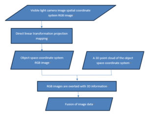
In the detection and imaging system, the images of the visible light camera are in the image space coordinate system, and the 3D point cloud data obtained by single photon detection is in the object space coordinate system. During imaging, the corresponding pixels in 2 different spaces follow a collinear equation:
\[\label{e1} \left\{\begin{array}{l} x-x_0=-f \frac{a_1\left(X-X_s\right)+b_1\left(Y-Y_s\right)+c_1\left(Z-Z_s\right)}{a_3\left(X-X_s\right)+b_3\left(Y-Y_s\right)+c_3\left(Z-Z_s\right)}, \\ y-y_0=-f \frac{a_2\left(X-X_s\right)+b_2\left(Y-Y_s\right)+c_2\left(Z-Z_s\right)}{a_3\left(X-X_s\right)+b_3\left(Y-Y_s\right)+c_3\left(Z-Z_s\right)}, \end{array}\right. \tag{1}\] where, \((x,y)\) are the coordinates of each pixel of the visible light camera in the pixel coordinate system; \(({x_0},{y_0})\) is the image principal point coordinate of the visible light camera; \(f\) is the focal length of the visible light camera; \((X,Y,Z)\) are the coordinates of the 3D point cloud data; \(({X_s},{Y_s},{Z_s})\) is the coordinates of the visible light camera photography center in the object space coordinate system; \(\left[\begin{array}{lll} \mathrm{a}_1 & \mathrm{a}_2 & \mathrm{a}_3 \\ \mathrm{~b}_1 & \mathrm{~b}_{\mathrm{z}} & \mathrm{b}_3 \\ \mathrm{c}_1 & \mathrm{c}_2 & \mathrm{c}_3 \end{array}\right]\) is the directional cosine in the spatially varying rotation matrix.
The basic formula for the coordinate conversion of the two-dimensional image of the visible light camera and the corresponding image point in object space can be obtained by direct linear transformation:
\[\label{e2} \left\{\begin{array}{l} x+\frac{l_1 X+l_2 Y+l_3 Z+l_4}{l_9 X+l_{10} Y+l_{11} Z+1}=0, \\ y+\frac{l_5 X+l_6 Y+l_7 Z+l_8}{l_9 X+l_{10} Y+l_{11} Z+1}=0. \end{array}\right. \tag{2}\]
Considering nonlinear factors such as image distortion, the image point coordinates can be expressed as follows:
\[\label{e3} \left\{\begin{array}{l} x=f_x\left(l_1, l_2, l_3, l_4, l_5, l_6, l_7, l_8, l_9, l_{10} l_{11}, X, Y, Z\right), \\ y=f_y\left(l_1, l_2, l_3, l_4, l_5, l_6, l_7, l_8, l_9, l_{10}, l_{11}, X, Y, Z\right). \end{array}\right. \tag{3}\]
According to the direct linear transformation model in the formula, there are a total of 11 positional parameters to be solved in the process of projection transformation of the whole system, which include 3 internal azimuth elements, 6 external azimuth elements, 1 coordinate axis non-orthogonal coefficient, and 1 coordinate axis proportional inconsistency coefficient of the imaging system [13].
\[\label{e4} V = BL – X , \tag{4}\]
\[\label{e5} L=\left(B^T P B\right)^{-1} B^T P X . \tag{5}\]
Due to the large size of objects that are close to the lidar and the size of objects that are far away are relatively small, the size of the target is not uniform. After converting the point cloud to voxel form, there is a quantization loss of the original point cloud data features [14,15]. Therefore, whether it is the original point cloud data or the voxelized data, it will affect the accuracy of 3D object detection.
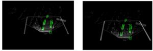
In the Bird’s Eye View (BEV), there is almost no occlusion because the viewpoint is raised, the receptive field in the z-axis direction becomes larger, and there are fewer obstacles. In addition, the target size is more uniform in the bird’s-eye view, and there is no phenomenon of near large and far small. Secondly, a bird’s-eye view is a two-dimensional image with a regular arrangement of pixels, which can be calculated with the help of a two-dimensional image-based processing method. The following illustration illustrates the conversion of a point cloud from a front view to a bird’s-eye view, where the resolution is set to 0.05 meters during the conversion (see Figure 2).
The goal of neural network training is to find the optimal set of network parameters to minimize the value of the loss function, and if there is large-scale training data, the robustness and accuracy of the network model will be directly improved. In the dataset, there are only 7481 annotated training samples, so the original training data is enhanced using pseudo-sampling, ground truth target random perturbation, and global scaling.
Pseudo-sampling is the random insertion of ground truth objects and truth boxes from one scene into another new scene. Specifically, firstly, the target objects, corresponding labels, and truth boxes in the training dataset are extracted to form a new database [16,17]. Then, for each frame of the point cloud, several ground truth targets are randomly sampled from the constructed database and inserted into the point cloud of the current frame. Finally, compare whether the newly inserted truth box coincides with the existing truth box in the current frame, and if it does, discard the target corresponding to the truth box. The effect of the point cloud before and after pseudo-sampling is shown in the figure below, compared with before sampling, the number of ground truth targets in the same frame point cloud is greatly increased, so the pseudo-sampling method can simulate complex scenes and improve the generalization ability of the network (see Figure 3).

In order to reduce the impact of noise on network performance in real-world scenarios, rotation and noise are applied randomly and independently to each ground truth target. where the angle of rotation is (\(\pi\),\(2\pi\)) and the noise is sampled from a standard Gaussian distribution with an expected 0 and a standard deviation of 1. The enhancement method of random perturbation of ground truth targets can make the network more adaptable in the new environment, and the figure below shows the effect of applying rotation and noise to ground truth targets (see Figure 4).
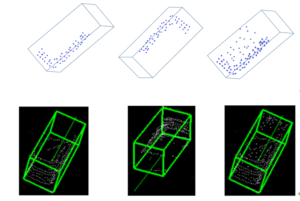
In real-world scenarios, targets such as vehicles, pedestrians, and riders may not be of the same size compared to the targets in the training set. Therefore, the whole point cloud and the ground truth target are scaled to the coordinates of each point in the point cloud \((x, y, z)\), the coordinates of the ground truth box \(({x_t},{y_t},{z_t})\), and the size of the ground truth box \((l, w, h)\), and the magnitude of the zoom is \(\alpha\) and the value is taken from the uniform distribution \(\alpha \in\) [0.9,1.1]. The effect before and after scaling is shown in the following figure, where a takes a value of 1.1 (see Figure 5).
Five key indexes, including compression information, compression/solution efficiency, compression/solution time, compression/solution format, and restoration quality, were selected to analyze four typical point cloud compression algorithms. Table 1 shows the comparison results of typical point cloud compression characteristics.
| Compress | Compress | Compress/Decompress | Compress/Decompress | Compress/Decompress | Restore |
| Algorithm | Information | Efficiency | TimeFormat | Quality | |
| Draco | Geometry + Attributes | Poor | Medium | .pcd | Controllable |
| HEV | CGeometry | Better | SLow | .bin | Undamaged |
| Realtime | Geometry + Depth | Better | Quick | .bin | Damaged |
| BitPan | Geometry +Color | Better | Slow | .bin | Damaged |
Comparing the four compression algorithms of Draco, HEVC, Realtime and BitPan, it can be seen that only the Draco algorithm has the ability to compress geometry and multiple attributes, in which the attribute information includes texture, color, normal and other information, while some other compression algorithms only support geometric information, and some only support a single attribute information, and the compression of multiple point cloud attribute information is of great significance for the high restoration of the environment: In terms of compression solution efficiency, the compression efficiency of the Draco algorithm is inferior compared with other methods, because Draco focuses on the compression of multi-attribute information, and does not optimize and improve the compression objects of the characteristics. In terms of compression solution time, except for the Realtime algorithm, the compression real-time performance of other compression algorithms is not good [18,19]. In terms of compression deformatization, the four compression algorithms only support the compression of point cloud files in .bin or. pcd formats, which is not conducive to improving the real-time compression of files: in terms of restoration quality, only the compression parameters of the Draco algorithm can be controlled.
In summary, although the compression/solution efficiency of the Draco algorithm is not high, and the compression/solution time is not fast, it has the advantages of compressing a variety of attribute information and controllable restoration quality, which makes it very suitable for improvement and optimization.
The Draco algorithm uses the octree model to encode dense point clouds, which has good robustness, but due to the uneven collection equipment and environment, some of the point cloud data collected are far away from the core area, that is, outliers. However, the octree algorithm will build a model based on the entire point cloud set in the spatial envelope, and the existence of outliers makes it difficult to model the octree. In order to solve this problem, this paper clips and filters the point cloud set before constructing the octree to optimize the point cloud compression model. The specific cropping and filtering effects are shown in Figure 6.
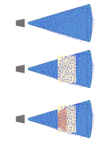
Clipping point cloud set: Clipping is mainly done by determining the core area \(X[{x_{\min }},{x_{\max }}]\), \(Y[{y_{\min }},{y_{\max }}]\), and \(Y[{y_{\min }},{y_{\max }}]\), where \(Y[{x_{\min }},{x_{\max }},{y_{\min }},{y_{\max }},{z_{\min }},{z_{\max }}]\) represents the maximum and minimum values of the \(x, y, and z\) axes in the point cloud spatial coordinate system, respectively, and the removal of discrete points is completed by determining the cropping threshold.
Filtered point cloud gathering: Mainly aiming at the problem of sparse distribution of local point clouds in the pruned space, the filtering process calculates the average distance and variance between a single point cloud and all point clouds in the neighborhood except itself. The threshold was determined according to the Gaussian morphological distribution of the mean distance and variance of the point cloud, and finally the point cloud exceeding the threshold part was filtered.
If it is to suppose there are a total of point clouds after clipping, let the cloud coordinates of a certain point be \(I({x_1},{y_1},{z_1})\), and there are \(M\) points in the neighborhood with a radius of \(S\), and the average distance from point \(I\) to these \(M\) points is;
\[\label{e6} \varepsilon^1=\frac{1}{M} \sum_{m=1}^M\left(x_1-x_m\right)^2+\left(y_1-y_m\right)^2+\left(z_1-z_m\right)^2 . \tag{6}\]
The mean distance is
\[\label{e7} \sigma=\frac{\varepsilon^1+\varepsilon^2+\varepsilon^3+\cdots+\varepsilon^n}{n} . \tag{7}\]
The variance is
\[\label{e8} \delta=\mathrm{E}\left[\sum_{\mathrm{i}=1}^{\mathrm{n}}\left(\sigma-\varepsilon^1\right)^2\right] . \tag{8}\]
It is assumed that the average distance of the point cloud \(\alpha\) obey a Gaussian distribution: \(\alpha ~N(\sigma ,\delta )\). Let \(\varepsilon '\) be the boundary value of the confidence interval, i.e., the confidence interval is \([ – \varepsilon ',\varepsilon ']\).
Hypothesis \(A \in (0,1)\) The threshold set for the user, which means the probability value of the confidence interval. \(\varepsilon '\) is found by Eq. (9).
\[\label{e9} \int_\sigma^{\varepsilon^1} f(a) d a=\frac{A}{2} \Rightarrow \varepsilon^1 . \tag{9}\]
The range to be filtered is obtained from \(\varepsilon '\) , and the points whose average distance is outside the threshold are defined as non-core points, and the non-core points are filtered out.
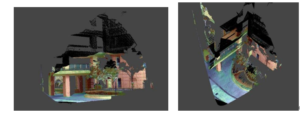
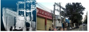
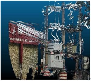
In this paper, LDAR-DP software is used to fuse the original image and idar point cloud data. After comparing the color point cloud with the original image data, the color point cloud was evenly distributed, and there was no miscorrespondence, dislocation and stretching with the equipment in the station area, and the image and point cloud registration effect was good. According to the experimental results, the color point cloud production technology based on the image matching method still has a good registration and fusion effect in the scene of the distribution network area, which can truly reflect the panoramic sense and texture characteristics of the ground objects, which proves that the technology has strong robustness and high adaptability, and the effect is shown in the Figure 7.
Raw 3D point clouds and 2D images of visible light acquired by photon detection imaging systems (see Figure 7 and 8).
The three-dimensional data with RGB information is superimposed by fusion processing as shown in 8.
After using the bounding box to preliminarily determine whether there is a possible overlapping area between each viewing angle, the method proposed in this paper is used to estimate the overlap rate between any two viewing angles, and the weight calculation result of each side (keeping three significant places after the decimal point) is shown in Table 2:
| – | View 1 | View 2 | View 3 | View 4 | View 5 | View 6 |
| View 1 | – | 3.139 | 0.725 | 27.949 | 19.196 | 1.523 |
| View 2 | 3.139 | – | 1.022 | 4.367 | 18.7697 | 10.412 |
| View 3 | 0.725 | 1.022 | – | 1.029 | 4.768 | 35.298 |
| View 4 | 27.949 | 4.367 | 1.029 | – | 0.819 | 5.298 |
| View 5 | 19.196 | 18.7697 | 4.768 | 0.819 | – | 1.216 |
| View 6 | 1.523 | 10.412 | 35.298 | 5.298 | 1.216 | – |
In order to verify the robustness of the RCS-Draco algorithm in compressing the colored point cloud stream algorithm in real time, this paper compares the compression level and quantization level set by changing the compression decompression efficiency and compression solution time in the design process of the RCS-Draco algorithm in the same point cloud scenario, so as to show the characteristics of the RCS-Draco algorithm with controllable compression and reduction quality [20].
The first parameter of the RCS-Draco algorithm, “Level”, is used to adjust the compression decompression speed and compression desolution rate, and the general compression level can be changed between 0 10, in order to compare the influence of the compression level on the compression parameters, a total of 4 parameters equal to 0, 3, 7 and 10 are selected for horizontal comparison.
The second parameter of the RCS-Draco algorithm, “Quantify”, is used to represent the degree to which geometric and attribute information is quantized, the smaller the quantization number (except 0), the lower the quantization level of the unit data, the higher the relative compression ratio, and the greater the compression error. In particular, when the quantization standard is 0, it means lossless compression, that is, maintaining the complete accuracy of the point cloud data. Generally, the level of quantification can vary between 0 20. In order to compare the influence of quantization level on the compression parameters, a total of 4 parameters were selected for longitudinal comparison, including 0, 5, 10 and 15.
The output time of the point cloud packet is 310 s, the output frequency is 10 Hz, the total number of msgs is 370, and the size is 773.7 MB.
The experimental results are shown in Table 3 to Table 5.
| Quantative Level | L=0/ACR/% | L=0/APE/m | L=0/ACE | L=3/ACR/% | L=3/APE/m | L=3/ACE | L=7/ACR/% | L=7/APE/m | L=7/ACE | L=10/ACR/% | L=10/APE/m | L=10/ACE |
| Q=0 | 15.428 | 16.754 | 15.753 | 17 325 | 15.113 | 19.951 | 13.948 | 17.262 | 17 325 | 15.113 | 19.951 | 17 325 |
| Q=5 | 28.542 | 13.344 | 26.655 | 12 .937 | 23.130 | 14.387 | 21.800 | 15.562 | 12 .937 | 23.130 | 14.387 | 12 .937 |
| Q=10 | 34.387 | 17.802 | 32.178 | 18. 327 | 27.653 | 17.140 | 20.956 | 15.723 | 18. 327 | 27.653 | 17.140 | 18. 327 |
| Q=15 | 34.799 | 19.793 | 34 840 | 18. 306 | 28 845 | 19,598 | 24,602 | 17,124 | 18. 306 | 28 845 | 19,598 | 18. 306 |
| Quantative Level | L=0/ACR/% | L=0/APE/m | L=0/ACE | L=3/ACR/% | L=3/APE/m | L=3/ACE | L=7/ACR/% | L=7/APE/m | L=7/ACE | L=10/ACR/% | L=10/APE/m | L=10/ACE |
| Q=0 | 77.003 | 0.000 | 6.413 | 75.003 | 0.000 | 6.413 | 75.003 | 0.000 | 6.366 | 75.003 | 0.000 | 6.413 |
| Q=5 | 1.193 | 0.018 | 34.478 | 1. 193 | 0.048 | 34.478 | 1.294 | 0.048 | 34.478 | 4.001 | 0.048 | 34.292 |
| Q=10 | 10.989 | 0.003 | 4.087 | 10.989 | 0.003 | 7.087 | 11 922 | 0.003 | 7.087 | 12.438 | 0.003 | 7.087 |
| Q=15 | 22.058 | 0.000 | 6. 860 | 22.058 | 0.000 | 6.860 | 23 643 | 0.000 | 6.860 | 18.477 | 0.000 | 6.812 |
| Quantative Level | L=0/ACR/% | L=0/APE/m | L=0/ACE | L=3/ACR/% | L=3/APE/m | L=3/ACE | L=7/ACR/% | L=7/APE/m | L=7/ACE | L=10/ACR/% | L=10/APE/m | L=10/ACE |
| Q=0 | 72.003 | 1.000 | 6.433 | 72.003 | 1.000 | 3.413 | 35.003 | 1.000 | 3.366 | 65.003 | 1.000 | 5.413 |
| Q=5 | 0.193 | 1.018 | 33.478 | 0. 193 | 1.048 | 24.478 | 3.294 | 1.048 | 34.478 | 5.001 | 1.048 | 24.292 |
| Q=10 | 11.989 | 1.003 | 5.087 | 11.989 | 1.003 | 1.087 | 21 922 | 1.003 | 2.087 | 22.438 | 1.003 | 1.087 |
| Q=15 | 21.058 | 1.000 | 3.860 | 12.058 | 1.000 | 3.860 | 13 643 | 1.000 | 2.860 | 28.477 | 1.000 | 2.812 |
It can be seen from Table 2 that under the same compression level (e.g., L=3), as the quantization level increases from 5 15, the ACR increases sequentially, and the APE and ACE decrease sequentially: when the quantization level is 0, the ACR is the maximum. This shows that the average compression ratio can be effectively changed by changing the quantization level, but the corresponding average compression error will also increase. However, under the same quantization level (e.g., Q=10), with the increase of compression level from 1 10, the ACR increased slightly, and there was no significant change in APE and ACE. This shows that under the same quantization level, changing the compression level can only change the average compression ratio, and will not affect the compression error. It can be seen from Table 3 that under the same compression level (e.g., L=3), ACT and ADT both increase sequentially as the quantization level increases from 5 15, which indicates that increasing the quantization parameters will increase the average compression and decompression time. When the quantization level is 0, the ACT is the smallest and the ADT is the largest, which indicates that lossless compression does not quantize, reducing the compression time but increasing the decompression time. However, under the same quantization level (e.g., 0=7), ACT decreases as the compression level increases from 1 10, and ADT fluctuates in a small range. This shows that increasing the compression level will not only lead to an increase in the average compression ratio, but also a decrease in the compression time, and the decompression will fluctuate in a small range with the change in compression difficulty.
It can be seen from Table 4 that under the same compression level, the restoration degree and clarity of the image increase successively as the quantization level increases from 5 15. The quantization parameter with the highest degree of reproduction is 0, that is, lossless compression, which indicates that controlling the quantization parameter can effectively change the sharpness and reproduction of the image. However, under the same quantization level, with the increase of the compression level L from 1 10, the restoration and clarity of the image are not significantly improved, which indicates that the method of changing the compression level has no obvious effect on improving the restoration and clarity of the image.
On the whole, compared with the HEVC and real-time algorithms, which cannot effectively adjust the compression performance, the RCS-Draco algorithm can control the average compression ratio to change between 1 77%, the average error of position and color can change between 0 0.05 m and 4 35b, and the average compression and decompression time is 13 35 ms and 12 20 ms by adjusting the compression level and quantization level. Experimental results show that the RCS-Draco algorithm can change the compression ratio, compression error, compression and decompression time by adjusting the compression parameters, and the controllability and flexibility of compression are better than those of HEVC and real-time algorithms.
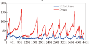
In order to verify the optimization effect of the RCS-Draco algorithm proposed in this paper compared with the Draco algorithm , an ablation experiment was also set up to analyze the improvement results of the RCS-Draco algorithm compared with the Draco algorithm under the five evaluation parameters of ACR, APEACE, ACT, and ADT under the same scenario and the same compression parameters. In order to unify and compare the experimental parameters, the dataset selected for this experiment was the point cloud dataset in the outdoor environment (0ut-door), the output time of the point cloud packet was 533 s, the output frequency was 10 Hz, and the total number of MSGS was 4 525, and the occupancy size was 8.5 GB. The uniform compression level is equal to 5, and the quantization level 0 is equal to 10.
As can be seen from Figure 9, the compression time of the RCS-Draco algorithm (blue) is lower than that of the Draco algorithm (red) in the ACT aspect, and the compression time of the former is less than 100 ms in the whole compression process, which is less than 10 Hz of the message receiving frequency, and the compression time of Draco often fluctuates greatly. This is not conducive to the transmission and decompression of point cloud data. As can be seen from Figure 10, in terms of ADT, the decompression time of RCS-Draco (blue) is slightly lower than that of Draco’s algorithm (red), and it can be seen that the former has a certain improvement in decompression time compared with the latter.
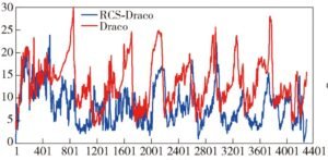
In this paper, a new multi-view point cloud stitching method is designed, and the technology in it is theoretically studied, and the point cloud based on GPGPU is fused to the point cloud, which greatly improves the speed of point cloud fusion. The RCS-Draco algorithm is better than the Draco algorithm in the main indexes of compression (ACR, APE, ACE, ACT, ADT), which proves that the RCS-Draco algorithm proposed in this paper is superior to the Draco point cloud compression algorithm and has strong robustness and stability in the real-time compression of point clouds. The RCS-Draco algorithm is a compression method mainly for point cloud stream data, which mainly encodes point cloud stream data with color, and the encoding process is controllable and effective, and is better than similar compression methods.
Research on the application of on-site operation safety behavior pre-control device based on spatio-temporal synthesis technology.