
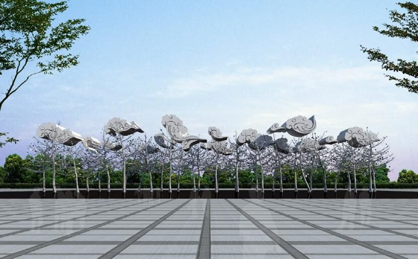
Installation display space art design in exhibition spaces has gained increasing attention as a critical element in enhancing the viewer’s experience. Unlike traditional two-dimensional art forms, installation art utilizes three-dimensional space to create immersive, interactive environments that engage the audience both physically and emotionally. This form of art has expanded significantly, integrating elements from architecture, sculpture, and digital media to transform exhibition spaces into dynamic and thought-provoking environments [1,2].
The evolution of installation art design has been influenced by advancements in technology, particularly in areas like virtual reality and 3D modeling, which allow artists to conceptualize and present their works in innovative ways. In the design of exhibition spaces, these technologies help create visually engaging installations that harmonize with the spatial environment, emphasizing aesthetics, functionality, and user experience [3,4].
Through strategic placement, material selection, and consideration of spatial interaction, installation art can influence how visitors move through and perceive an exhibition. This has led to a growing demand for installation art design that not only reflects the artistic vision but also enhances the functionality and sustainability of the exhibition space. The interplay between art, space, and technology forms the core of modern installation art design, making it a vital component in shaping contemporary cultural and artistic environments [5,6].
Among them, interaction, realism, diffusion, functionality and usage are the five main indicators of software evaluation, and their hierarchical ordering and relative weights are shown in Table 1.
| Evaluate | Interactivity | Authenticity | Functionality | Usage degree | Extensibility | Relative weight | Hierarchical sorting |
| Interactivity | 1 | 7 | 6 | 8 | 8 | 0.583 | 1 |
| Authenticity | 1/7 | 1 | 4 | 6 | 5 | 0.212 | 2 |
| Functionality | 1/6 | 1/4 | 1 | 4 | 4 | 0.116 | 3 |
| Usage degree | 1/8 | 1/6 | 1/4 | 1 | 1 | 0.055 | 4 |
| Extensibility | 1/8 | 1/5 | 1/4 | 1 | 1 | 0.049 | 5 |
Natural landscapes are mainly composed of mountains, lakes, rivers, oceans, earth, trees, flowers, plants, clouds, smoke, fog and other natural geometric features. Since these landscapes are naturally occurring, their geometries are irregular, which makes it extremely difficult to simulate natural environments with computers in real-time realism. The rapid development of fractal theory provides an effective means for the simulation of natural landscape [7,8]. In this paper, based on the basic principles of Lindenmayer Systems, random midpoint displacement method and particle systems in fractals as theoretical basis, we analyze and study the current fractal modelling and simulation techniques for 3D modelling of plants, 3D terrain generation, as well as for natural landscapes such as clouds, smoke, fog, flames, forests, meadows and oceans [9].
The use of binocular vision stereo camera to establish a three-dimensional terrain scene of the landscape, the use of Sketch UP software to establish a three-dimensional tree model, all the required elements of the landscape design model to build the completion of the landscape design elements and the use of Unity3D engine will be completed the design of the garden scene to display to the user.
Virtual three-dimensional visual technology into the design of landscape simulation system, the system development process needs to be clear through the garden design unit of the different aspects of landscape design and functional requirements, based on the needs of landscape design system modules, so that the designed system has a high degree of practicality [10]. The overall structure of the designed virtual three-dimensional visual technology installation art design in exhibition halls simulation system is shown in Figure 1.
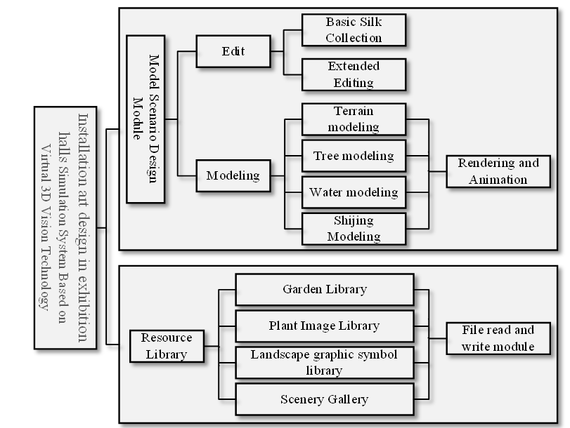
The display space designed system mainly consists of two parts: model scene design module and resource library. The model scene design module includes editing and model building two parts, the use of editing part of the system to achieve different operations editing, model building part of the system includes terrain modelling, tree modelling, water modelling and stone landscape modelling four parts, each part of the model building is completed through the rendering and animation part of the model built to achieve the integration of the integrated model, after the integration of the model that is, the final design of the garden landscape results [11]; Through the resource library to provide resource support for the system, the resource library, including garden library, plant picture library, garden plane symbol library, with the scene picture library four parts, the garden landscape design process needs to call the relevant resources, the use of file reading and writing module will be the resources converted to the required format, easy to access the system [12].
The binocular stereo vision camera is represented by \({x_c}\) , \({l^T},{e^T},{v^T},{\omega ^T}\) denote the rotational quaternion, coordinate position, linear velocity and angular velocity of the camera, respectively, and the camera state equation can be obtained as follows:
\[\label{e1} {x_c} = {\left( {{l^T},{e^T},{v^T},{\omega ^T}} \right)^T}.\tag{1}\] The 3D world coordinates of the camera map feature state vector using the feature points to form the camera map are \({g_i}{\left( {{x_i},{y_i},{z_i}} \right)^T}\) . \[\label{e2} x = {\left( {x_c^T,g_1^T,g_2^T,…,g_i^T,…,g_n^T} \right)^T}.\tag{2}\] \[\label{e3} \mathbf{x}_{\mathrm{c}, t+1}=\left[\begin{array}{c} e_{t+1} \\ l_{t+1} \\ v_{t+1} \\ \omega_{t+1} \end{array}\right]=\left[\begin{array}{c} e_t+\left(v_t+m_v\right) \Delta t \\ l_t \times l\left(\omega_t+m_\omega\right) \Delta t \\ v_t+m_v \\ \omega_t+m_\omega \end{array}\right],\tag{3}\] where \({\left[ {{m_v},{m_\omega }} \right]^{\text{T}}}\) denotes the process noise during the reconstruction of the 3D terrain scene.
The coordinates of the projected position of the random point \(Q\) within the reconstructed 3D terrain scene within the image are given in the following formula:
\[\label{e4} \left\{\begin{array}{l} x=\frac{g X_c}{Z_c}, \\ y=\frac{g Y_c}{Z_c}. \end{array}\right.\tag{4}\] The coordinates of the observations in the captured image using feature points matching the map feature points are represented in the following equation:
\[\label{e5} D = {({D_1},{D_2},…,{D_n})^T},\tag{5}\] where \(m\) and \({D_i} = ({u_i},{v_i})\) denote the number of matched feature points and the coordinates of the acquired image when the feature point is \(i\) , respectively.
Add the measurement noise\({u_i}\) to Eq. (e5) to obtain the measurement equation as follows:
\[\label{e6} \mathbf{D}_i=\left[\begin{array}{l} u_i \\ v_i \end{array}\right]+\mu_i=\left[\begin{array}{l} \frac{g_u \times x_{i c}}{z_{i c}}+u_0 \\ \frac{g_v \times y_{i c}}{z_{i c}}+v_0 \end{array}\right]+\mu_i.\tag{6}\] Style: \[\label{e7} \left[\begin{array}{c} x_{i c} \\ y_{i c} \\ z_{i c} \end{array}\right]=K * \mathbf{X}^{\mathrm{w}}+t,\tag{7}\] where, \(({g_u},{g_v})\) and \(({u_0},{v_0})\) denote the focal length and optical, respectively; \(K,t\) denotes the external parameters; \({({x_{ic}},{y_{ic}},{z_{ic}})^T}\) and \({{\bf{X}}^{\text{W}}}\) denote the coordinates of the feature point in the binocular stereo vision camera coordinates and in the world coordinate system, respectively.
Based on the binocular stereo vision camera position \(({g_t},{l_t})\) , the feature point position in world coordinates is initialized based on the 3D coordinates of the feature point in camera coordinates.
Setting \({e_{n + 1}}\) as the new feature point, the formula for the variance of this point under the camera can be obtained as follows:
\[\label{e8} {{\bf{Q}}_{{X_{{\text{RCGB}}}}}} = \left( {\theta _{{x_{{\text{R}}G\;{\text{B}}}}}^2,\theta _{{y_{{\text{RCCB}}}}}^2,\theta _{{z_{{\text{RCB}}}}}^2} \right),\tag{8}\]
\[\label{e9} {f_{n + 1}} = K\left( {{l_t}} \right){X_{{\text{RGB}}}} + {e_t},\tag{9}\] where, \({\theta _{{x_{{\text{RCB}}}}}},{\theta _{{y_{{\text{RCB}}}}}},{\theta _{{z_{{\text{RCGB}}}}}}\) denotes the standard deviation of the desired reconstructed scene in different directions within the binocular vision stereo camera coordinates and \(X\) and \(Q\) denote the state vector and covariance of the added feature point, respectively. It can be obtained that after adding this feature point, the binocular vision camera state of the reconstructed 3D terrain scene is transformed into:
\[\label{e10} Q^{\prime}=\left[\begin{array}{cc} Q & Q\left(\frac{\partial g_{n+1}}{\partial x}\right)^{\mathrm{T}} \\ \frac{\partial g_{n+1}}{\partial x} Q & AP \end{array}\right],\tag{10}\] where
\(AP=\frac{\partial g_{n+1}}{\partial x} Q\left(\frac{\partial g_{n+1}}{\partial x}\right)^{\mathrm{T}}+\frac{\partial g_{n+1}}{\partial X_{\mathrm{RGB}}} Q X_{\mathrm{RGB}}\left(\frac{\partial g_{n+1}}{\partial X_{\mathrm{RGB}}}\right)^{\mathrm{T}}\).
When the number of visible reconstructed point clouds from the binocular stereo vision camera is less than the total number of pixels 2 3 during the 3D reconstruction of the terrain scene localization process, the external parameter \({T_{cw}} = \left[ {{K_{cw}},{t_{cw}}} \right]\) is used to set the 3D point clouds from the binocular vision camera within the world coordinates, so as to realize all the 3D reconstruction of the visible point clouds from the camera.
Plants are living matter, the existence of randomness, singularity and complexity of the growth process, while the plant species are diverse, and the morphology of different species of plants is very different. These characteristics of plants should be fully considered in 3D modelling of plants [13].
The L-system, known as the regular display space system, outside, is a character parallel generalization of the plant growth process and abstract construction of axioms (representing plant seeds) and generative sets (describing the plant’s growth rules) [14]. In order to build a complete and effective plant model, L-systems have been continuously extended with deterministic L-systems (D0L), stochastic L-systems, parametric stochastic L-systems, and context-dependent stochastic parametric L-systems. With the help of these L-systems, various morphologies of various plants and various characteristics during plant growth, such as plant pruning, plant phototropism and geotropism, are realistically modelled by constructing L-systems representing plant seeds and describing the growth rules of plants. As in Figure 2, plants generated by constructing different L-systems are shown, where (a) is a plant with normal morphology; (b) is the structure of a plant drawn after adding pruning factors to (a); (c) is a plant with normal morphology; (d) is the morphology change when the phototropic feature is obvious with respect to (c); (e) is the morphology change when the geotropic factor is large with respect to (c); and (f) is the structure of a plant with long flowers, fruits, and leaves.

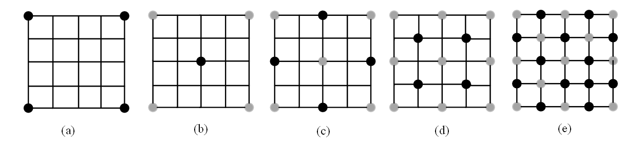
Using the midpoint displacement method on a two-dimensional plane, called the 2D random midpoint displacement method, it is possible to simulate three-dimensional random fractal terrain using the 2D random midpoint displacement method. In this method, the core of the rectangle or square is displaced and the displaced height value is used as the new vertex, the rectangle or square is divided into four new rectangles or squares, the midpoint is then computed on each of the new rectangles or squares and the displacement is added to iterate repeatedly [15]. As shown in Figure 3, the four corners were set to the same height, and the four corners of (a) were given initial height values, indicated by black dots.
The computation at each step of the iteration can be summarized by the following equation:
\[\label{e11} {X_n}(x,y) = {f_n}(x,y) + {\Delta _n}*\operatorname{Gauss}.\tag{11}\]
The offset added at each step is a random variable with a Gaussian distribution with variance: \(\Delta _{\text{n}}^2 = {\left( {\frac{1}{2}} \right)^{{\text{nh}}}}{\sigma ^2}\) . Where \({{\text{X}}_{\text{n}}} = ({\text{x}},{\text{y}})\) denotes the value of current point \(({\text{x}},{\text{y}})\) , the location of viewpoint \(({\text{x}},{\text{y}})\) , \(\operatorname{Gauss} ()\) denotes a Gaussian random number that follows a normal distribution. The shape of the mountain range with different roughness can be obtained by controlling \({\Delta _n}\) .
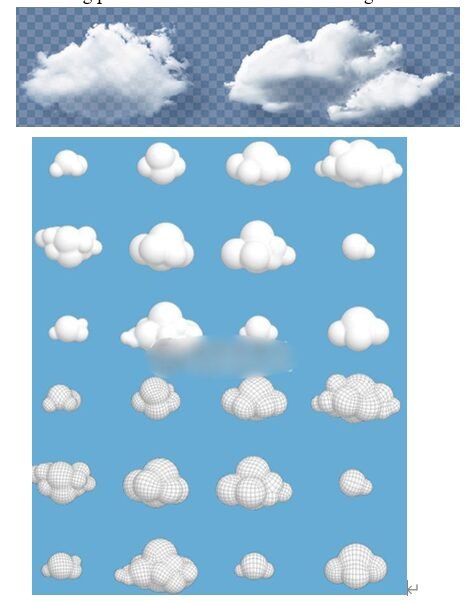
Natural phenomena such as clouds, smoke, fog, flames, etc. are difficult to realize their real-time simulation in simulation systems using the FBM (Fractional Brownian Motion) method and the L-system method due to their irregularity, dynamics and randomness. Particle systems are by far considered to be one of the most successful graph generation methods for simulating irregular dynamically changing objects . Particle systems have been successfully applied to the simulation of natural phenomena such as clouds, smoke, fog, flames, forests, meadows, oceans and so on, and dynamic real-time simulation of these natural phenomena has been achieved. The following is an example of cloud to illustrate the modelling and simulation techniques of such natural landscapes.
The basic shape of the cloud can be defined as a simple ellipsoid then certain deformations are made to these cloud spheres in all different directions and the initial cloud sphere is randomly scaled down and randomly replicated several times at small displacements away from the of the cloud sphere in different orientations, continuing until the last iteration, and finally the scaled sphere is drawn . In the modelling process, the fractal process is simplified and improved by treating the particles of the cloud directly as particles of the particle system, which has data information such as position, radius, color and transparency. The following discussion focuses on how to determine the position and radius of cloud particles using fractal techniques. The coordinates of the core of the cloud are \({\left( {X,Y,Z} \right)_{\text{ }}}\) , and the radius of the cloud is \(R\) . The position of the cloud particles offsets this core randomly, and its radius \(r\) is a number obtained by multiplying the distance to the core by a random interval that is \(\left[ {0,1} \right]\). (Eq. (e12) is the position formula and Eq. (e13) is the radius formula. The base color of the cloud particles can be set to a uniform amount set to the color under no influence of light.
\[ \text{Cloun}{d_i} \cdot {\text{X}} = {\text{X}} + {\text{R}} \times \text{Randam}(i),\tag{12}\]\[ \text{Cloun}{d_i} \cdot {\text{Y}} = {\text{Y}} + {\text{R}} \times \text{Random}(i),\tag{13}\] \[ \text{Cloun}{d_{\text{i}}} \cdot {\text{Z}} = {\text{Z}} + {\text{R}} \times \text{Randam}(i).\tag{14}\] And the radius of the cloud particles can be expressed as:
\[\label{e14} {C_{{r_i}}} \ne {\text{R}} \times \Delta {{\text{L}}_{\text{i}}} \times {\text{}}\text{Random}(i),\tag{15}\] where \(\Delta {{\text{L}}_{\text{i}}}\) denotes the distance of the cloud particle from the core of the cloud.
The fractal modelling process of the cloud is shown in Figure 4.
In order to give a realistic appearance to the cloud, the intensity of the color of the cloud ball is considered as a function of its height above the ground, with the color becoming more intense the closer the ball is to the ground, and gradually becoming lighter as the height increases.
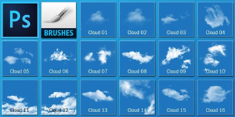
When real-time simulation of clouds is achieved with a particle system, each particle represents a cloud mass, represented by a quadrilateral, mapping a 2D texture to a planar polygon and making that polygon always face the position of the observation point, thus creating a three-dimensional sense of a planar object, and generating a realistic sea of clouds through image synthesis and the multiple rendering technique in OpenGL . As in Figure 5.
Visual Studio 2010 is selected as the system development platform and is used as the development language to develop the system of this paper. Selected a city of a community landscape design as a system to verify the object, the community is located in the southeast of the city, is a newly developed ecological district, the district covers a total area of 13,854 \({m^2}\), with a total construction area of 18,564 \({m^2}\), the residential area contains a total of nine residential buildings, including villas, multilayer and high-rise areas, the landscape design requirements for the district greening area of more than 35%.
Three-dimensional terrain scene modelling in landscape design is an important part of the landscape design contains numerous building information, with a large amount of modelling, the difficulty is high, selected binocular stereo vision camera used in this paper to establish the three-dimensional terrain scene model of the district as shown in Figure 6. The three-dimensional terrain scene model established by the binocular stereo vision camera can include all the architectural information and road information of the landscape project to be reconstructed, and the reconstructed three-dimensional terrain scene model and the actual building can be presented at a ratio of 1:1, which is convenient for the designers to add the information of landscape elements in the future.
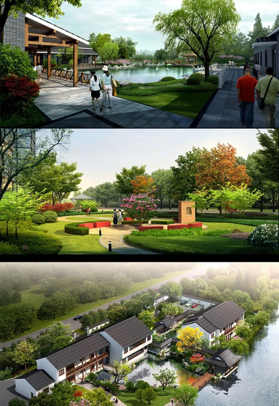
The water body model established using the system in this paper is shown in Figure 7. The water body is an important part of the garden landscape, the water body exists in static and dynamic forms, the establishment of the water body model needs to be based on different forms of water body to establish a different structural model, the use of this paper’s system can be effectively established in the design of the garden landscape dynamic water model, the establishment of the water body model has a high degree of fidelity, which can effectively reflect the effect of the dynamic water body, the simulation results verified that this paper’s system has a high degree of water body modelling The simulation results verify that the system in this paper has high water modelling performance.
Using the model in this paper to establish the stone model within the garden landscape is shown in Figure 8. The use of this system can effectively achieve the establishment of stone models within the landscape design scene, stone is an important part of the composition of the landscape, the use of a large number of stones to form an artistic road as well as stone scenery, can reflect the artistic nature of landscape design. The system can effectively establish different shapes and materials of stones, and use the established stone model to build a large area of stone scenery.
The system can design landscapes according to the specific characteristics of the experimental objects of the required landscaping design, which effectively reduces the labor intensity of the landscaping designers and shortens the design cycle. The garden landscape designed using the established 3D terrain scene model is more accurate than the 2D garden landscape design, and the accuracy of the garden landscape design is effectively enhanced because the 3D terrain scene model is established with 1:1 ratio. The system in this paper can design the landscape from a human point of view within the 3D scene model.
Hierarchical analysis method is selected to evaluate the effect of systematic design of garden landscape in this paper, hierarchical analysis method is a multi-objective decision analysis method combining quantitative and qualitative, which is extremely suitable for evaluation factors that cannot be quantified. The results of using hierarchical analysis to evaluate the garden landscape designed by the system in this paper are shown in Table 2. From the evaluation results in Table 2, it can be seen that using hierarchical analysis to evaluate the final effect of the garden landscape designed by this paper’s system through 10 indicators such as graphic refresh rate, visual brightness, visual contrast, etc., with an average score of 94.7, and the scoring results indicate that this paper’s system has a high degree of design effectiveness.
| Evaluating indicator | Weight | Evaluation results/points |
| Graph Refresh rate | 0.2346 | 96 |
| Visual Brightness | 0.0855 | 97 |
| Visual contrast | 0.0952 | 98 |
| Resolving power | 0.0864 | 92 |
| Stereo | 0.0576 | 93 |
| Shadow processing | 0.1686 | 94 |
| Illumination | 0.0829 | 95 |
| Special effects | 0.0716 | 94 |
| Model Scale | 0.0639 | 92 |
| Location correspondence | 0.0547 | 96 |
| Average value | – | 94.7 |
Fractal theory is an effective tool for simulating natural landscapes. Fractal recursive algorithms and L-systems excel in virtual plant simulation, fractional Brownian motion is ideal for 3D terrain modeling, and particle systems are highly effective for simulating irregular, dynamic objects like clouds, smoke, flames, and oceans. Virtual 3D vision technology and binocular stereo cameras enhance immersion and realism in garden landscape design by reconstructing 3D terrains. The system effectively simulates a community garden, demonstrating high spatial utilization, fidelity, and well-integrated visual effects.
This research is supported by the Social Science Foundation of Jiangsu Province, China (No. 24YSD009),Project Leader (Yongjun He).