
With the rapid pace of technological development, smart electronic devices are becoming increasingly common and essential in daily life. Despite advancements that enhance the quality of these products, prolonged usage often leads to wear and malfunctions. Moreover, as systems grow in both investment and scale, their complexity increases. Interconnected components within devices create intricate relationships, where a fault in one part can trigger a cascade of issues, potentially disrupting entire systems [1,2]. In industrial settings, predicting faults presents formidable challenges, necessitating swift and effective decision-making in conditions characterized by high measurement noise, extensive data correlations, voluminous inputs, and intricate symptom-fault interactions.
Point processes are often used in time series to better model real-world scenarios [3]. Among these, temporal point processes are stochastic processes that consist of events occurring in a continuous time domain, such as sequences of events (e.g., predicted earthquake occurrences, train arrival times, user website visits, and customer arrival times). The Poisson and Hawkes processes are the most typical models in traditional time-series point processes.
With the advancement of neural networks and deep learning, these techniques have been widely recognized and utilized across various fields. For instance, [4,5] treat the intensity function of a point-in-time process as a non-linear function of historical data and use recurrent neural networks (RNNs) to learn the historical impact of events automatically. In [6], event sequences and time sequences in time-point processes are modeled using two recurrent neural networks to predict event timings and classify event types. Generic continuous time series models proposed in [7,8] aim to learn the influence relationships between different events in an event stream and predict both the timing and type of future events. These methods have been applied in diverse areas such as healthcare analysis, smart cities, consumer behavior, and social network prediction.
The increasing complexity and integration of electronic devices in today’s society highlight the necessity of robust and proactive fault prediction methods. Timely identification of potential faults is essential for improving device reliability, minimizing downtime, and reducing maintenance costs. This study presents a novel method for predicting electronic device faults by combining 2D and 3D image analysis techniques with a time-series point process based on an attention mechanism [9,10].
Conventional time series forecasting techniques are straightforward and universal, but they suffer from lags and produce predictions that are insufficiently precise [11]. While traditional point process methods are highly interpretable, their accuracy often depends on the selected point process function. These methods rely on a relatively small number of samples, leading to reduced prediction accuracy. Furthermore, there is a risk of manually selecting an incorrect model [12].
The focus of this article is on electronic device fault prediction. To address the issues of overestimation during stable periods and underestimation during decline periods in existing fault rate prediction models, a time-point process generation model based on a self-attention mechanism is proposed. This approach aims to improve both the prediction accuracy and the interpretability of the model.
The self-attention mechanism illustrates the interdependencies between input data using a one-to-one similarity function. The query-key-value self-attention paradigm is used in this paper, and the precise computation procedure is as follows:
Each of the \({\boldsymbol{e}}_n \in E = \left[e_1, \cdots, e_N\right] \in \mathbb{R}^{L \times N}\) inputs is linearly mapped to three distinct spaces. The query vector \(q_i \in \mathbb{R}^D\), the key vector \(k_i \in \mathbb{R}^D\), and the value vector \(v_i \in \mathbb{R}^D\) are obtained. For the entire input sequence \(E\), the linear mapping process is \[\begin{aligned} Q &= E W_q = \left[q_1, \cdots, q_D\right] \in \mathbb{R}^{L \times D}, \\ K &= E W_k = \left[k_1, \cdots, k_D\right] \in \mathbb{R}^{L \times D}, \\ V &= E W_v = \left[v_1, \cdots, v_D\right] \in \mathbb{R}^{L \times D}, \end{aligned}\] where \(W_q \in \mathbb{R}^{N \times D}\), \(W_k \in \mathbb{R}^{N \times D}\), \(W_v \in \mathbb{R}^{N \times D}\) are the parameter matrices for the linear mappings.
The output vector corresponding to the self-attention mechanism for each query vector (\(q_n \in Q\)), key vector (\(k_j \in K\)), and value vector (\(v_j \in V\)) is given by: \[h_n = \sum_{j=1}^N a_{nj} v_j = \sum_{j=1}^N \text{softmax} \left( s(q_n, k_j) \right) v_j,\] where \(a_{nj}\) indicates the weight of the \(n\)-th input in relation to the \(j\)-th input, \(s(\cdot)\) is the similarity function, \(\text{softmax}(\cdot)\) is the normalizing function, and \(n, j \in [1, N]\) are the positions in the sequence of input vectors.
The output sequence is \(H = \left[h_1, \cdots, h_D\right] \in \mathbb{R}^{L \times D}\). The self-attention mechanism can be thought of as establishing the interaction between elements in a linear projection space. However, to capture distinct interactions across multiple projection spaces, multiheaded self-attention is employed in \(M\) projection spaces, where \(\forall m \in \{1, \cdots, M\}\): \[\begin{aligned} Q &= E W^m_q, \\ K_m &= E W^m_k, \\ V_m &= E W^m_v, \\ H &= \left[h_1, \cdots, h_D\right] W_0, \end{aligned}\] with \(W_0 \in \mathbb{R}^{N \times D}\), \(W^m_q \in \mathbb{R}^{N \times \frac{D}{M}}\), \(W^m_k \in \mathbb{R}^{N \times \frac{D}{M}}\), \(W^m_v \in \mathbb{R}^{N \times \frac{D}{M}}\) as the projection matrices.
Given a vector \(Z = \left\{z_1, z_2, \cdots, z_L\right\} \in \mathbb{R}^{L \times 1}\) as input data, the position encoding vector \(p(z_t) \in \mathbb{R}^{L \times N}\) is predefined as follows: \[\label{GrindEQ__3_} {\left[p\left(z_j\right)\right]}_i = \begin{cases} \sin \left(\frac{pe\left(z_j\right)}{10000^{\frac{i-1}{M}}}\right), & i \, \text{is even}, \\ \cos \left(\frac{pe\left(z_j\right)}{10000^{\frac{i-1}{M}}}\right), & i \, \text{is odd}, \end{cases} \tag{1}\] where \(pe(z_j)\) represents the position (order) of \(z_j\) in the input sequence. This encoding method enriches the location information without introducing additional parameters, thereby improving the model’s capability to utilize positional data effectively.
This paper proposes a point-in-time process generation method that combines the multi-head self-attention mechanism and Wasserstein distance [13] to improve the learning effect of point-in-time process generation, capture the long-range dependencies of event sequences, and make the distribution of generated sequences closer to real sequences. Figure 1 illustrates the structure of the model, which consists of a generative network and a discriminative network with components such as positional encoding, multi-head self-attention, residual connection, layer normalization, fully connected layers, and a softmax layer [14].
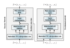
The following describes the individual components of the model:
With an input sequence of \(Z = \{z_1, z_2, \ldots, z_L\}\) and an output sequence of \(X = \{x_1, x_2, \ldots, x_L\}\), the generative network seeks to transform the noise sequence into a series of events that the discriminative network is unable to distinguish, i.e., \(g_\theta(Z) = X\). The generative network samples the noise sequence from a Cartesian Poisson process, which is uniformly distributed and non-informative.
A self-attention mechanism lies at the core of the generative network to compensate for the lack of timestamped position information in the input sequence. An embedding encoding \(e(\cdot) \in \mathbb{R}^{L \times N}\) combined with a positional encoding \(p(\cdot) \in \mathbb{R}^{L \times N}\) forms \(E = [e(z_1) + p(z_1), \ldots, e(z_L) + p(z_L)], E \in \mathbb{R}^{L \times N}\), which corrects the input noise sequence \(Z = \{z_1, z_2, \ldots, z_L\} \in \mathbb{R}^{L \times 1}\) by incorporating positional encoding. The multi-head self-attention mechanism processes the encoded sequence and uses the scaled dot product as a similarity function to produce the output \(H = [h_1, h_2, \ldots, h_M] W^0 \in \mathbb{R}^{L \times 1}\), where \[h_m = \text{softmax}\left(\frac{Q_m K_m^T}{\sqrt{D_k}}\right) V_m.\]
To prevent future events from influencing the current step, a masking mechanism is applied during the self-attention process. Specifically, when calculating the \(j\)-th row (\(Q_m K_m^T(j,:)\)) of the matrix \(Q_m K_m^T\), values such as \(Q_m K_m^T(j, j+1)\), \(Q_m K_m^T(j, j+2)\), \(\ldots\), \(Q_m K_m^T(j, L)\) are set to negative infinity. After softmax processing, this ensures that the influence of future events on the current event is zero, so only historical events affect each event. Furthermore, layer normalization successfully prevents the gradients from vanishing or exploding, and residual connections are introduced in the multi-head self-attention output to mitigate degradation issues caused by increased model depth. Ultimately, the multi-head self-attention’s output \(H\) is passed through the fully connected layer to produce the output sequence \(X = \{x_1, x_2, \ldots, x_M\} = \sigma(H W^f + b^f)\), where the activation function \(\sigma(\cdot)\) represents \(ELU(\cdot)\), \(X \in \mathbb{R}^{L \times 1}\), \(W^f \in \mathbb{R}^{L \times 1}\), and \(b^f \in \mathbb{R}^{L \times 1}\).
The discriminative network’s role is to determine whether the input sequence comes from the generative network or real data. Except for the final layer, the discriminative network has a structure identical to the generative network. The output of the final layer, softmax, is used to construct a loss function that calculates the difference between the generated and real sequences [15].
To validate the model presented in this work, cases from the literature were selected for comparative analysis. Table 1 provides the relevant failure rate statistics for 58 SFPSZ9-120,000/220 transformers collected from the literature.
| Serial Number of Transformer | Service Life (Years) | Failure Rate (times/(set $$\cdot$$ year)) | Serial Number of Transformer | Service Life (Years) | Failure Rate (times/(set $$\cdot$$ year)) |
| 13 | 4.5 | 0.0144 | 42 | 18.8 | 0.0239 |
| 14 | 4.6 | 0.0127 | 43 | 18 | 0.0331 |
| 15 | 5 | 0.0227 | 44 | 19.6 | 0.0575 |
| 16 | 6 | 0.0114 | 45 | 21 | 0.0434 |
| 17 | 7.3 | 0.0139 | 46 | 20.6 | 0.0557 |
| 18 | 7.5 | 0.0132 | 47 | 22 | 0.0682 |
| 19 | 7.6 | 0.0142 | 48 | 23 | 0.0448 |
| 20 | 7.8 | 0.0233 | 49 | 24 | 0.0606 |
| 21 | 7 | 0.0207 | 50 | 23.6 | 0.0762 |
| 22 | 8 | 0.0185 | 51 | 25 | 0.0887 |
| 23 | 9 | 0.0155 | 52 | 24.6 | 0.0995 |
| 24 | 10 | 0.0186 | 53 | 24.9 | 0.0965 |
| 25 | 12 | 0.0168 | 54 | 25 | 0.1021 |
| 26 | 12.3 | 0.0151 | 55 | 25.4 | 0.1156 |
| 27 | 12.4 | 0.0155 | 56 | 26 | 0.1341 |
| 28 | 13 | 0.0135 | 57 | 26.6 | 0.1144 |
| 29 | 13.6 | 0.0358 | 58 | 27 | 0.1504 |
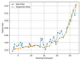
Table 1 shows that random factors significantly impact the raw transformer fault data. The outliers are smoothed using the median filtering approach to determine the fault cut-off points [16]. The smoothing technique only considers the fault data for the entire year, and median filtering replaces the outliers with the median value in the anomaly data domain. A sliding window with five values was used for filtering, considering the sample size and the one-dimensional nature of the fitted fault curves [17,18]. Figure 2 displays the results of the data smoothing process.
MATLAB programming was utilized to perform the curvature valuation computation procedure described in Section 3.1.2. When selecting line segments, it was ensured that the starting point ratio for each segment was zero. Necessary modifications were made to guarantee all initial points exceeded the difference between the cut-off points. The data was divided into groups of six, with the subsequent group beginning at the penultimate number of the preceding group, ensuring all data could be effectively compared, as shown in Figure 3.
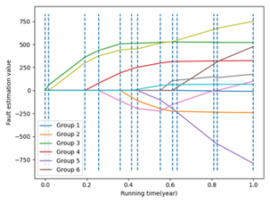
The points lie on the line segments connecting the data set’s start and end points if their curvature value is zero. Each data set contains local maxima, as shown in Figure 3. Expert experience identifies the distinctive points at \(t = 16\), \(t = 22\), \(t = 23\), \(t = 24\), and \(t = 25a\). The threshold value \(t_v\) is 0.35. Based on the morphological features of the electrical equipment melting pool curve, the following inferences can be made:
The failure rate increases after the fault demarcation point, whereas the data prior to the demarcation point exhibits a smooth trend.
There is only one fault demarcation point. Therefore, it can be concluded that the boundary between the transformer fault stabilization period and the fault loss period is at \(t = 16a\).
To validate the model’s accuracy, the gray linear regression model and the fault assessment model based on the Marquardt method (abbreviated M-R algorithm) were selected for comparative analysis. The prediction outcomes based on the Marquardt algorithm are as follows:
\[\begin{aligned} \lambda (t) = \begin{cases} 0.0169, & t \leq 15a, \\ \frac{4.551}{28.1719} \cdot \left(\frac{t}{28.1719}\right)^{3.551}, & t > 15a. \end{cases} \end{aligned} \tag{2}\]
The gray linear regression model predicts outcomes as: \[\begin{aligned} \begin{cases} \hat{y}^{(0)}(t+1) &= \hat{y}^{(1)}(t+1) – \hat{y}^{(1)}(t), \\ \hat{y}^{(1)}(t) &= 5.0714e^{0.1859t} + 9.8231t – 8.0204. \end{cases} \end{aligned} \tag{3}\]
Due to the large sample size of the case data, comparing the prediction accuracy of the three models in a table format is infeasible. Instead, the relative errors between the measured and predicted values for each of the three models were calculated as:
\[e_j = \frac{y_j – x_j}{x_j}, \tag{4}\] where \(y_j\) represents the expected value, \(x_j\) is the measured value, and \(e_j\) is the relative error rate. Figure 4 displays the error test results for each model.

An error rate of zero denotes the baseline. A positive relative error rate indicates that the expected value is higher than the actual value, while a negative error rate indicates the opposite. The extreme fluctuations in the curves in Figure 4 illustrate how sporadic electronic device failures influence predictions. The fluctuation amplitudes of the three curves differ significantly, with Curve 3 being closer to the baseline, despite similar fluctuation trends. When no data segmentation is performed, data during the stabilization period is influenced by depletion period data, leading to larger predictions, while data during the depletion period is influenced by stabilization data, resulting in smaller predictions. Consequently, Curve 1 is primarily above the baseline during the stabilization period and below the baseline during the depletion period.
The R05 gearbox in a factory contains five shafts with four pairs of gears meshing inside. A variable-frequency motor with a rotational speed of approximately 1017 r/min drives the input, and after four stages of deceleration, the output rotates at roughly 5 r/min. The test conditions are as follows: the motor rotational speed is 1017 r/min, the sampling frequency is 704 Hz, the number of sampling points is 8192, and the test data file name is 2002112142048, which specifies the time of data collection. Vibration signals of a pair of gears meshing on the VI and V shafts with a meshing frequency of 369 Hz are measured at measurement point 3, situated in the vertical direction of the fifth axis gearbox housing [19,20]. The VI and V shafts, along with their gear pairs, frequently experience malfunctions due to various reasons, which in extreme cases can cause damage to the shafts or gears. Below, the data collected at measurement point 3 will be analyzed and compared.
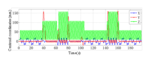
The results of the empirical modal decomposition for the data at measurement point 3 are shown in Figure 5. While Figure 5b presents the amplitude spectrum analysis of the corresponding signals, Figure 5a illustrates the time-domain waveforms of the decomposed modal functions, including the original signal and the first six intrinsic modal components arranged from top to bottom.
The original signals are processed using the empirical modal decomposition method based on the decomposed modal functions and vibration modes, as shown in Figure 5. The main frequencies of im4 are 111 Hz and 74 Hz, corresponding to three and two times the meshing frequency of 369 Hz, respectively. The main frequency of im5 is 74 Hz, reflecting two times the vibration mode of the meshing frequency. Additionally, the center frequency is 338 Hz, which corresponds to the vibration mode at twice the motor rotational speed. Moreover, other frequency components modify the primary frequencies of im4 and im5, indicating that the gear meshing process reveals the shock impact caused by gear failure or load variation.
This paper proposes a time point process generation model based on the Wasserstein distance and a multi-head self-attention mechanism for predicting electronic device faults. The self-attention mechanism enhances the model’s interpretability and generalization by effectively capturing long-distance relationships in event sequences, without relying on fixed form strength functions, as conventional methods do. Built on the structural design of generative adversarial networks, this method optimizes the generated sequence through discriminative networks, approximating the true distribution and improving prediction accuracy.
Experimental results demonstrate that the proposed model performs well in predicting transformer failure rates, achieving a relative error reduction of 3.59% and a prediction accuracy improvement of 3.91% compared to traditional methods, thereby fully verifying the model’s effectiveness and superiority. Furthermore, the introduction of the masking mechanism and position encoding technology enhances the model’s performance in processing complex time series data, providing an innovative solution for fault prediction.
The authors would like to sincerely thank those who contributed techniques and support to this research.
The experimental data supporting the findings of this study are available from the corresponding author upon request.
The authors declare that they have no conflicts of interest regarding this work.
This work was supported by the Scientific Research Key Fund of Hunan Provincial Education Department (No. 22A0574).