In the realm of information security, malware detection in IoT environments is crucial. This research proposes a heterogeneous graph network based malware classification model to enhance the detection and categorization of sophisticated malware samples. The model is composed of five primary modules: a module for building heterogeneous graphs; a module for generating random wandering sequences; an aggregation module based on LSTM; a module for wandering based on attention mechanisms; and a module for classification and prediction. Initially, a heterogeneous graph comprising API and malware nodes is built, and using random wandering, the associations between far-off nodes are obtained to improve the representation of node features. Next, using the attention mechanism, LSTM is utilized to aggregate the data of nodes on various paths, learn how different paths affect nodes, and ultimately output the node categorization results through the linear layer. The model performs better in terms of precision, recall, and F1 value than conventional techniques like Node2Vec, GCN, and GraphSAGE, according to the trials done on the APIMDS and Mal-API-2019 datasets. Furthermore, by inserting, removing, and changing pointless API calls, robustness tests are carried out to confirm the model’s resilience to malware variants.
Internet of Things (IoT) technology is expanding quickly and is being used extensively across a range of businesses in the current digital era [1]. But as the number of IoT devices has increased, malware has spread widely, presenting a severe risk to information security. Malware compromises data security and personal privacy by entering Internet of Things devices, controlling device operations, and stealing sensitive information. This can have a major negative impact on the economy and society in addition to being a threat to data security [2]. As a result, it is crucial to investigate and create effective malware detection methods [3].
The two primary categories of malware detection strategies are behavior-based and signature-based approaches. Signature-based techniques detect malware by comparing feature libraries of known malware, which works well against known threats but is less successful in identifying novel malware types and variations [4]. Behavior-based approaches, which have some flexibility and generalization power to identify unknown malware, identify whether a piece of software is malware by examining its operating behavior. Nevertheless, as malware technology has advanced, its concealed and sophisticated behavioral patterns have created additional difficulties for behavior-based detection methods [5,6].
Current strategies for behavior-based malware detection primarily depend on static and dynamic analysis methodologies. Static analysis parses binary data and software code to extract features, but it has trouble handling methods like encryption and code obfuscation. By mimicking the software’s running environment and keeping an eye on its system calls, network activity, etc., dynamic analysis is able to extract features. While it can partially address the drawbacks of static analysis, it still has issues including a large overhead and a sluggish detection speed [7,8]. Additionally, as deep learning technology advances, an increasing number of researchers are using it to identify malware. By automatically extracting features and patterns through the learning of a vast quantity of sample data, deep learning improves detection resilience and accuracy. However, it is challenging to properly utilize the structural relationship information across samples because standard deep learning methods mostly rely on the feature vector representation of samples [9].
This research suggests a malware classification methodology based on heterogeneous graph networks to overcome the aforementioned issues [10]. By building a heterogeneous graph with malware and API nodes and using methods like random wandering and LSTM aggregation to thoroughly explore the structural relationships and node features among samples, the model increases the accuracy and robustness of malware detection and classification. In particular, this contribution primarily focus on the following areas:
In order to create a heterogeneous graph with malware nodes and API nodes, malware and the API call sequences associated with it are chosen as study items [11,12]. A graph structure that may accurately depict the behavior of malware is created by streamlining the API call sequences, eliminating consecutively repeated API calls, cutting down on the graph’s complexity, and keeping the most important behavioral aspects.
In order to retrieve the complete feature representation of the current node, the LSTM model is utilized to perform feature aggregation on many pathways created by random wandering and capture the sequence information of the nodes on the paths.When processing sequence data, LSTM performs well and may efficiently combine data from several pathways to increase feature representation accuracy.
Furthermore, this work designs adversarial tests of insertion, deletion, and replacement of useless APIs to confirm the robustness of the model. The findings demonstrate that, in comparison to more conventional approaches, the model presented in this research is more robust and stable when handling malware variations and more successful at thwarting malware evasion detection techniques.
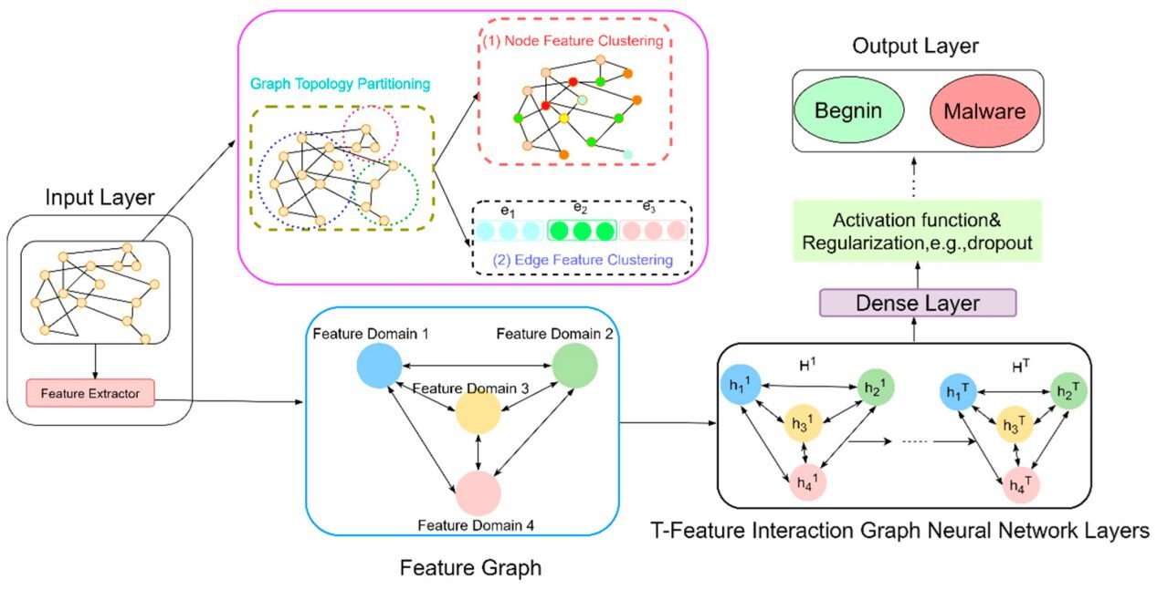
The five modules that make up our suggested malware classification model based on heterogeneous graph networks are the attention-based wandering module, the LSTM-based aggregation module, the random wandering sequence generating module, the heterogeneous graph construction module, and the classification and prediction module [13]. First, we decide to create a heterogeneous graph with these two kinds of nodes in order to categorize malware samples based on two links between malware and APIs and API functions in API call sequences [14]. We use random walks to find distant “neighbor” nodes of the nodes in order to capture the relationship between malware and distant malware and APIs in the heterogeneous graph. This allows us to use the information of distant nodes to obtain the feature representation of the current node. LSTM is used to aggregate the feature information of each path in order to obtain the final node representation by combining the node information on many paths. In the meantime, the attention mechanism is used to learn the embedding results of various paths in order to employ the impacts on the current node in various paths due to the existence of many different paths [15]. After running the acquired node representation through a linear layer, the node classification result is finally produced. Figure 1 depicts the overall model structure and methodology.
Since applications require APIs to access operating system functions at runtime, as was previously mentioned, extracting the API call sequences of software samples can accurately and intuitively represent the real behavior of the samples. For this reason, we choose to analyze the malware’s API call sequences as well as the malware itself [16]. A big heterogeneous graph is constructed with two types of nodes: malware and API, and the edges that result from their relationships. The call relationship between malware and API functions creates the edges between malware and APIs; that is, when malware calls an API, a MAL-API edge is created. We decide to simplify each software’s API call sequence by eliminating API subsequences that share consecutive API functions and usage patterns in order to shorten the length of API calls and reduce graph complexity [17,18]. Table 1 displays the streamlined procedure.The call order in the API sequence determines the API-API concatenation. The malware and API produce a heterogeneous graph based on the edge rule, as seen in Figure 2, where the blue nodes stand in for APIs, the other colors for software samples, and the nodes of various colors are thought to belong to distinct malware families. The MAL-API edge is shown by the black line between the software sample nodes and API nodes, and the API-API edge is represented by the blue line between the API nodes.
| Initial API order | Simplified API sequence |
| \(A_1A_2A_2A_2A_1\) | \(A_1A_2A_1\) |
| \(A_1A_2A_3A_1A_2A_3\) | \(A_1A_2A_3\) |
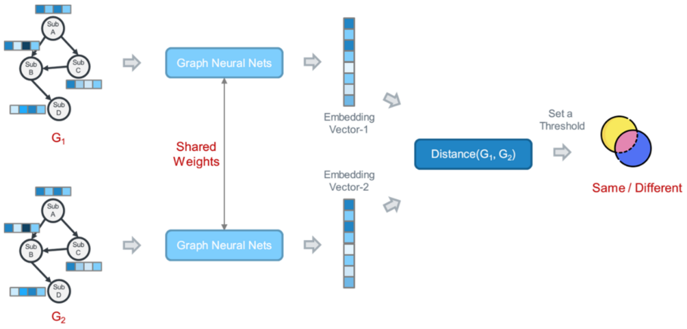
Thus, \(G\) can be defined as follows for the isomorphic graph that was built above:
\[\label{e1} G = (V,E). \tag{1}\]
If the malware node \({V_M}\) and the API node \({V_A}\) are concatenated to form the set of nodes \(V:\)
\[\label{e2} V = {V_M} \cup {V_A}. \tag{2}\]
The two types of edges—Api-Api connected edges and Mal-Api linked edges—that are defined in this study are included in the collection of edges \(E\).
\[\label{e3} E = \left( {{V_M} \times {V_A}} \right) \cup \left( {{V_A} \times {V_A}} \right). \tag{3}\]
All nodes are initialized using a normal distribution, represented by the number \(X = \left\{ {{x_1},{x_2},{x_3}, \ldots ,{x_n}} \right\} \in {R^{n \times d}}\), where \(d\) is the node’s vector dimension after embedding and \(n\) is the number of nodes.
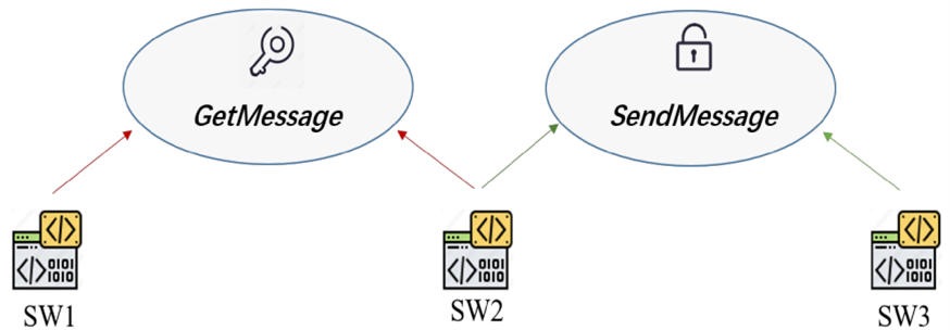
Unknown malware varieties can be categorized with the use of these correlations since malware may have certain associations with contacting certain common security-related or behaviorally different API methods. As illustrated in Figure 3, if software samples SW1 and SW2 call GetMessage, then both samples of software samples SW1 and SW2 perform the operation of getting user information, and if samples of software samples SW2 and SW3 call SendMessage, then both samples of software samples SW2 and SW3 perform the operation of sending the specified message to the window, and GetMessage and SendMessage perform the operation of sending the specified message to the window. to some extent, it can be assumed that software samples SW1 and SW3 are connected in some way because of the window and the strong correlation between GetMessage and SendMessage. A “path” based on this relationship between the software samples and the API can be used to classify malware that is unknown to us. This “path” can be used to classify malware that is unknown by looking at the relationship between software samples and APIs.
Traditional graph-based nodes’ neighbors are typically characterized as being centered on the target node; nodes that are away from the center node might be considered their \(k\)-order neighbors. However, the majority of graph network-based techniques only take into account how the neighboring nodes’ information features affect the center node; they ignore the potential impact of the higher-order neighbors on the center node depending on the paths. For example, GCNs are typically only taken into account for shallow GCNs because multilayer convolution causes over-smoothing.
Using a randomized wandering based on Node2Vec, we will be able to find the implicit associations between the intermediate nodes of the sequence and based on the properties of the constructed heterogeneous graph. Each software sample node will be the central node, and depth-first and breadth-first by means of the parameters \(p,q\). With the malware node acting as the center node, a biased selection traversal is carried out to obtain the common information of API nodes that are closer to the malware node and malware nodes that are farther away from the malware node.
The preferred selection method for the node \(x\) that will be visited in the next step is shown in Eq. (3), where \({d_{tx}}\) is the shortest distance between the node \(t\) and the node \(v.\) This is illustrated in Figure 4 as an example Node2Vec model graph, assuming that the previous node \(t\) is the node \(v\) that is currently at node \(v\). For the next visited node, \(x,\) depth-first traversal is favored when \(p>1\) and \(q<1\), and breadth-first traversal is preferred when \(p>1\) and \(q<1\).
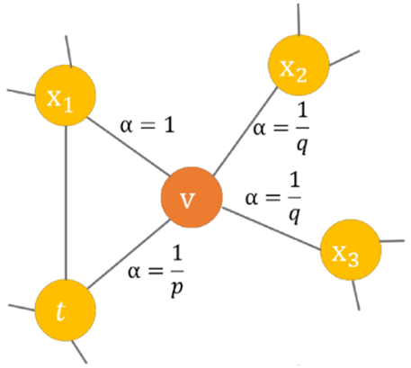
\[\label{e4} P\left(v_i=x \mid v_{i-1}=v\right)= \begin{cases}\frac{1}{p}, & d_{t x}=0, \\ 1, & d_{t x}=1, \\ \frac{1}{q}, & d_{t x}=2.\end{cases} \tag{4}\]
Since malware nodes have higher-order neighbors that are more likely to be malware nodes and first-order neighbors that are all API nodes due to the nature of the graph created, depth-first traversal is recommended to obtain information about isomorphisms as far away as possible. A traversal sequence of length \(\operatorname{Seq} = \left\{ {{v_{si}},{v_{s1}},{v_{s2}},{v_{s3}}, \ldots ,{v_{sk – 1}}} \right\}\) is produced by wandering. It is possible to think of every node \({v_{sj}},j = 1,2, \ldots k – 1\) in the sequence as a neighbor of node \({v_{si}}\).
The set of all sequence-based neighbors \({v_{si}}\) in the m-bar sequences obtained by node \({v_{si}}\) based on breadth-first and the set of all sequence-based neighbors \(N_i^D\) in the n-bar sequences obtained by node \({v_{si}}\) based on depth-first can be considered the neighborhood NB for the m- and n-bar sequences generated by node \({v_{si}}\) based on breadth-first and depth-first random wandering, respectively. the collection of all sequence-based neighbors \({v_{sj}}\) that node \({v_{si}}\) determined to be important in terms of depth.
Following processing using a linear layer, the outcomes of the multi-classification job are then mapped to the \((0,1)\) interval using softmax. The final classification result is determined by taking the highest classification probability.
\[\label{e5} {p_i} = \operatorname{softmax} \left( {{h_i} \cdot W} \right), \tag{5}\] where \({p_i}\) is the node i’s one-hot vector and \(W\) is the weight matrix. The cross-entropy loss function, which is specified as follows in the multi-classification job, is then used to optimize the model:
\[\label{e6} L = \frac{1}{N}\sum\limits_i {{L_i}} = – \frac{1}{N}\sum\limits_i {\sum\limits_{j = 1}^M {{y_{ij}}} } \log \left( {{p_{ij}}} \right), \tag{6}\] where \({y_{ij}}\) is the value when software \(i\) is projected to be in the actual category \(j\) and 0 otherwise, and \({p_{ij}}\) is the probability that software \(i\) is predicted to be in category \(j\). The number of observed software is represented by \(N\), the number of class labels by \(M\), and the categorization case by \({y_{ij}}\) is represented by \(M\).
Two datasets are used to pick the experimental datasets in order to fully measure the categorization effect of this model. The two datasets are the Mal-API-2019 dataset and the APIMDS dataset, which directly offer detailed information about the API call sequences and software sample type labels that are relevant to the task of malware multi-classification by using the call sequences that are suggested. The distribution of the various categories of data subset sets is displayed in Table 2. Of them, the APIMDS dataset comprises 23140 malwares, including 860 worms, 10847 Trojans, 580 backdoors, 960packers, 2350 adwares, 3130 other non-viruses, and 6710 other unlabeled data. 16,395 malware were deleted from the dataset after the unlabeled data had to be classified in order to create the malware families for the model.There are 7100 malware samples in the Mal-API-2019 dataset; Table 3 displays the distribution of malware categories and quantities in the dataset.
| Types of datasets | Subclass of dataset | Number | Total |
| Worm | P2P-worm | 50 | 850 |
| Worm | Email-worm | 90 | 850 |
| Worm | Net- worm | 130 | 850 |
| – | Trojan-Clicker | 20 | 10794 |
| – | Trojan-banker | 24 | 10794 |
| – | Trojan- Game Thief | 100 | 10794 |
| – | Trojan-dropper | 330 | 10794 |
| – | Trojan-downloader | 390 | 10794 |
| – | Trojan-ransomware | 440 | 10794 |
| – | Trojan-spy | 530 | 10794 |
| – | Trojan- PSW | 650 | 10794 |
| – | Trojan-fakeav | 3690 | 10794 |
| – | Trojan( Generic) | 3360 | 10794 |
| – | Others | 1260 | 10794 |
| Backdoor | – | 580 | 580 |
| Packed | – | 960 | 960 |
| Adware | – | 2350 | 2350 |
| Other | Webtoolbar | 210 | 780 |
| Other | DownLoader | 570 | 780 |
| Data-without-label | – | 6710 | 6710 |
| Types of datasets | Number |
| Adware | 370 |
| Backdoor | 1000 |
| Downloader | 890 |
| Dropper | 830 |
| Spyware | 1000 |
| Trojan | 1000 |
| Virus | 1000 |
| Worm | 1000 |
The Intel(R) Xeon(R) Gold 5122 CPU @ 3.60GHz, NVIDIA Corporation GP102 graphics card [GeForce GTX 1080 Ti], and Ubuntu 16.04.7 operating system are the tools used in this experiment. Python is the experimental language, while Pytorch is the deep learning framework that is used. Using the Pytorch deep learning framework, the language is Python.
This study’s model is the multiclassification model, which is assessed by comparing the actual data to the projected outcomes. A confusion matrix of dimension \(n× n\), where n is the number of software categories, will be produced as a result of the experiment. Because the experiment merely chose to categorize the dataset categories rather than breaking them down into more in-depth subclasses, the distribution of the number of subclasses of each type of malware sample in the dataset varies greatly, and some of the subclasses are minor. The following evaluation metrics are available for each category: the precision rate (P) for each category (K), recall (R), and F1 are the classical metrics used to assess the model in the classification task in the confusion matrix.
The F1 value metrics combine the results of the precision rate and recall rate. The precision rate is the ratio of the number of malware AC that truly belongs to category c to the number \(C{C_i}\) of all malware classified as C by this model, and the recall rate is the ratio of the number of malware TC of all malware TC belonging to category C to the number of malware classified as category C by this model \(C{C_i}\).
In the malware family categorization task, both macro- and micro-averaging metrics are applied to aggregate the detection findings for every family category. The global confusion matrix is used in micro-averaging to compute metrics like as precision, recall, and F1 value; that is, no sample in the dataset is classified. Each category is treated equally in macro-averaging, which then applies arithmetic averaging processes after determining the precision, recall, and F1 value metrics for each category independently.
In deep learning, the data is typically split into three categories: training, validation, and test sets. These sets are used to train the model, determine the model’s hyperparameters, and assess the model’s generalization effect, in that order. The training set will be used in the studies, and the test set will be 7:3. Using a variety of deep algorithms, including Node2Vec, GCN, and GraphSAGE, experiments will be carried out to assess the model’s detection capability as presented in this research. Every node in the heterogeneous graph is regarded as the same sort of node for Node2Vec, GCN, and GraphSAGE.
The value of \(p\) in depth-first based random wandering in the experiment is 10, the value of \(q\) is 0.1, and the value of \(p\) in breadth-first based random wandering is 0.1 in this model in order to highlight the propensity of depth-first and breadth-first based wandering. The value of \(q\) is 10. The studies select varying numbers of walks and maximum walk lengths for each node for comparison in order to obtain sufficient traversal paths and aggregate additional node features on the paths. Taking into account the performance issues, the final setting is to set each node’s maximum walk length and number of walks to 10. This is because when these parameters are small, the acquired sequence information is insufficient and the classification effect is poor, and when these parameters are large, the classification effect is hardly improved.
Two heads are used in the attention process in the tests.
Node2vec: This method converts nodes in a network into a dense low-dimensional vector representation by taking into account edges and edge weights between nodes. Neighboring nodes in the network receive comparable representations, and the original network topology is maintained throughout the representation process.
By employing a mix of depth-first and breadth-first strategies, Node2Vec generates a feature representation of every node in the graph through second-order random wandering. All of the experimental parameters are set to 10.
GCN: gathers data about core nodes’ first-order direct neighbors and can combine data from larger neighbors by stacking layers. Two GCN layers are put up in the experiment.
GraphSAGE: the experiment sets \(k=2\), and the aggregation function adopts the mean-value aggregation. Samples the kth-order neighbor nodes of each node in the graph, and updates the information of the nodes after aggregating the information of the nodes and the neighbor nodes according to the aggregation function (see Table 4, Table 5).
As shown in Table 3, KMO values are between 0.703, 0.7 and 0.8, and searching data is an appropriate method to extract information from more effective side effects.
| Algorithm | Precision/% | Recall /% | F1-score/% |
| Node2Vec | 94.89 | 94.56 | 96.23 |
| GCN | 96.14 | 96.52 | 95.48 |
| GraphSAGE | 96.54 | 96.52 | 96.58 |
| Proposed method | 95.28 | 97.48 | 96.25 |
| Algorithm | Precision/% | Recall /% | F1-score/% |
| Node2Vec | 95.25 | 96.12 | 95.24 |
| GCN | 96.12 | 95.62 | 95.25 |
| GraphSAGE | 96.54 | 96.25 | 98.24 |
| Proposed method | 96.58 | 96.85 | 96.88 |
Node2vec employs a random traversal of the graph, ignoring node feature information and concentrating more on the network structural relationship; as a result, its classification performs worse than the model in this study across all indexes; Similar to this, GraphSAGE-based methods can also improve the detection effect by taking node features into account, but they only capture the semantics of the second order neighbors. GCN-based methods take into account both the graph structural information and node feature information, which can improve the detection effect; however, they do not focus on the attention to different paths, so they are lower than this model in all the indexes. Comparatively, the GraphSAGE-based method also improves the detection effect by considering the node features, but it loses part of the information because it only captures the semantics of the 2nd-order neighbors; as a result, it is inferior to this model in all the indicators.
The GCN-based method considers both graph structure information and node features to improve the detection effect, but it does not pay attention to different paths. Based on the distribution characteristics of the nodes in the graph, the model, which is based on the LSTM aggregated attention mechanism for heterogeneous graphs, creates a heterogeneous graph with both API and malware nodes. Then, depth-first traversal and breadth-first traversal randomly wander to obtain different sequences, respectively, to obtain the information from the closer API nodes and the more distant malware nodes. The sequences are then aggregated based on various traversal techniques, and the multi-head attention mechanism is used to enable autonomous learning to determine the significance of each sequence to the center node. The models in this research achieve good results and have significant feature extraction capabilities for various datasets.
A comparison experiment of the robustness test is added in order to detect the function of inserting, deleting, and replacing useless APIs to avoid detection, as initially proposed by the model. On the one hand, the robustness of the malware deep learning model is of great significance in the detection of malware variants.
Under the condition of ensuring the normal operation of the original software function, this experiment selects three groups of useless {NtReadFile, NtOpenSection}, {NtOpenFile, NtWriteFile}, {NtOpenKey, NtCloseFile} as the perturbation objects and randomly inserts them into the original API call sequences according to the insertion perturbation rate in order to ensure that the insertion perturbation rate is approximately the same for each group of API call sequences.
Using {NtOpenKey, NtCloseFile} as the perturbation objects, choose the ineffective APIs at random based on the rate of insertion perturbation and then randomly add them back into the original sequence of API calls.
We employ the method of thoroughly counting the frequency of API functions in the API call sequence and verifying the API function definitions in order to identify the useless APIs in the original API call sequence. We then pick out the useless APIs and remove them based on the rate of perturbation, for example, API_useless={Sleep, IsWindow, lstrlenA, CreateFileW} and so forth. BuildFileW} and so forth.
Use (2) to identify the useless APIs in the original API call sequence. Then, choose API_useless from the list and replace it with APIs chosen from the useless API group depending on the rate of perturbation.
In order to achieve a perturbation rate of 0.02, 0.04, and 0.06, respectively, the experiment selects to inject 1 group, 2 groups, and 3 groups of pointless APIs into the data of API call length \(L=[100, 200, 300, 400, 500].\) Similarly, the corresponding number of groups of worthless APIs in the sequence are chosen for deletion and replacement, provided that the related perturbation rate remains constant.

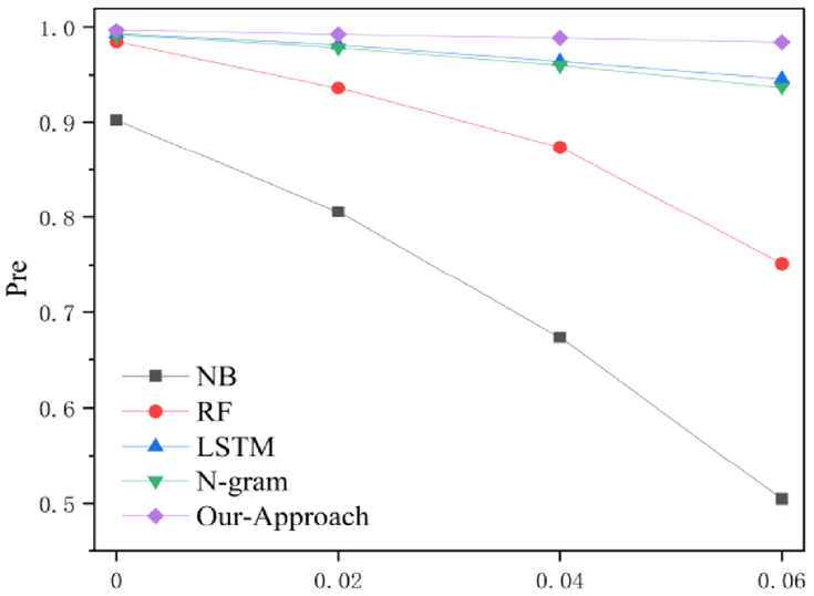
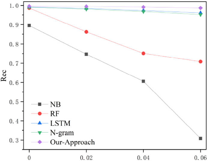
The performance changes of the other comparison techniques after inserting, removing, and replacing 1, 2, and 3 groups of pointless API perturbations, respectively, are depicted in Figure 5,Figure 6, and Figure 7. As can be seen in the picture, the shallow machine learning method’s metrics are much lower when compared to this model, and the fluctuation of malware detection metrics becomes more apparent after adding, removing, and replacing the disrupted API functions. As demonstrated in Figure 6, which displays the comparison results of the metrics after adding, removing, and replacing 1, 2, and 3 groups of pointless API perturbations to the ablation experiment model, the robustness of the ablation experiment is also tested. The blue and red color lines in the figure indicate the changes of the metrics of the ablation experiment and the model, respectively. The metrics of the ablation experiment and the model are found to be fairly comparable, but after the pointless API perturbation, the metrics of the model without the API correlation rule fluctuate more significantly (see Figure 8).

In this paper, we address the complex and dynamic malware threats in the IoT environment by proposing a malware classification model based on heterogeneous graph networks. By creating a heterogeneous graph with malware and API nodes, the model enhances the precision and resilience of malware detection and classification. It accomplishes this by utilizing techniques like random wandering and LSTM aggregation to fully exploit the structural relationships among samples and node features. The model presented in this research beats existing approaches like Node2Vec, GCN, and GraphSAGE in several metrics like classification accuracy, precision, recall, and F1 value, according to experimental results on the APIMDS and Mal-API-2019 datasets. To increase the effectiveness and resilience of malware detection, future study can investigate additional node feature kinds and associations, as well as enhance the model structure.
Ijaz, A., Khan, A. A., Arslan, M., Tanzil, A., Javed, A., Khalid, M. A. U., & Khan, S. (2024). Innovative machine learning techniques for malware detection. Journal of Computing & Biomedical Informatics, 7(01), 403-424.
Almazroi, A. A., & Ayub, N. (2024). Deep learning hybridization for improved malware detection in smart Internet of Things. Scientific Reports, 14(1), 7838.
Lee, H., Kim, S., Baek, D., Kim, D., & Hwang, D. (2023). Robust IoT malware detection and classification using opcode category features on machine learning. IEEE Access, 11, 18855-18867.
Jakkani, A. K., Reddy, P., & Jhurani, J. (2023). Design of a novel deep learning methodology for IOT botnet based attack detection. International Journal on Recent and Innovation Trends in Computing and Communication Design, 11, 4922-4927.
Kaushik, P. (2023). Unleashing the power of multi-agent deep learning: Cyber-attack detection in IoT. International Journal for Global Academic & Scientific Research, 2(2), 15-29.
Anitha, T., Aanjankumar, S., Poonkuntran, S., & Nayyar, A. (2023). A novel methodology for malicious traffic detection in smart devices using BI-LSTM–CNN-dependent deep learning methodology. Neural Computing and Applications, 35(27), 20319-20338.
Sasikala, S., & Sengathir, J. (2023). A review on machine learning-based malware detection techniques for Internet of Things (IoT) environments. Wireless Personal Communications 132. 1-14.
Wei, Y. Z., Md-Arshad, M., Samad, A. A., & Ithnin, N. (2023). Comparing malware attack detection using machine learning techniques in IoT network traffic. International Journal of Innovative Computing, 13(1), 21-27.
Venkatasubramanian, M., Lashkari, A. H., & Hakak, S. (2023). Iot malware analysis using federated learning: A comprehensive survey. IEEE Access, 11, 5004-5018.
Wang, X., Liu, J., & Zhang, C. (2023). Network intrusion detection based on multi-domain data and ensemble-bidirectional LSTM. EURASIP Journal on Information Security, 2023(1), 5.
Zhang, C., Roh, B. H., & Shan, G. (2023, December). Poster: Dynamic clustered federated framework for multi-domain network anomaly detection. In Companion of the 19th International Conference on emerging Networking EXperiments and Technologies (pp. 71-72).
Soliman, S., Oudah, W., & Aljuhani, A. (2023). Deep learning-based intrusion detection approach for securing industrial Internet of Things. Alexandria Engineering Journal, 81, 371-383.
Odeh, A., & Abu Taleb, A. (2023). Ensemble-based deep learning models for enhancing IoT intrusion detection. Applied Sciences, 13(21), 11985.
Gueye, T., Wang, Y., Rehman, M., Mushtaq, R. T., & Zahoor, S. (2023). A novel method to detect cyber-attacks in IoT/IIoT devices on the modbus protocol using deep learning. Cluster Computing, 26(5), 2947-2973.
Namasudra, S., Lorenz, P., & Ghosh, U. (2023). The new era of computer network by using machine learning. Mobile Networks and Applications, 28(2), 764-766.
Sarker, I. H., Khan, A. I., Abushark, Y. B., & Alsolami, F. (2023). Internet of things (iot) security intelligence: a comprehensive overview, machine learning solutions and research directions. Mobile Networks and Applications, 28(1), 296-312.
Munnangi, A. K., UdhayaKumar, S., Ravi, V., Sekaran, R., & Kannan, S. (2023). Survival study on deep learning techniques for IoT enabled smart healthcare system. Health and Technology, 13(2), 215-228.
Meddeb, R., Jemili, F., Triki, B., & Korbaa, O. (2023). A deep learning-based intrusion detection approach for mobile Ad-hoc network. Soft Computing, 27(14), 9425-9439.